If you’re interested in contributing a short What Am I Reading post, we’d love to hear from you! Email us at cache@colorado.edu.
Written by Jenna Tipaldo and Deborah Balk, CUNY Institute for Demographic Research
Researchers interested in studying the impacts of temperature on health face decisions on how to operationalize and measure exposures. This webinar “CAFE University: Considerations for temperature in public health studies” by Lauren Mock and Shreya Nalluri explores the myriad choices required when using temperature data to study health outcomes, from choice of metric and dataset to the study design.
The webinar includes an overview of various temperature metrics including land surface temperature (LST), air temperature (AT), heat index, wet bulb globe temperature (WGBT), and universal thermal comfort index (UTCI). A fuller discussion about choice of metrics can be found in this resource from the World Resources Institute (Engel et al. 2025), also referenced in the webinar. (It is useful to note that these are all measures of outdoor temperature. Measurement of indoor vs outdoor exposure is explored in another post on air pollution).
Each metric is more suited for specific purposes and contexts than for others, and each has drawbacks. For example, air temperature is widely available but doesn’t include factors that influence how humans perceive temperature, such as humidity. Both WGBT and UTCI do consider humidity.
Other dataset considerations include the availability of multiple metrics such as daily maximums, minimums, or averages. (All of the metrics discussed in the webinar provide daily temperature resolution, but some sensors have more fine-grain temporal data, such as hourly. See Table below.)
Additionally, researchers may choose to use raw temperature values versus standardized values such as percentiles, which can account for acclimatization.
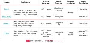
Source: CAFE University
Another aspect of operationalizing exposure is considering the timing of exposure relative to an outcome of interest – the webinar gives an example of defining the exposure period as the day of, day prior to, or three days prior to an event.
Even so, a recent paper (Cruz et al., 2025) proposes a framing of heat as a chronic phenomenon and argues that chronic exposures pose different risks that are not captured by existing research that evaluates the health impacts of acute exposures to extreme heat.
The webinar also explores the use of several gridded temperature datasets, including ERA5, gridMET, and PRISM, and how to link these with health data (e.g., calculating zonal statistics and population-weighting).
The webinar provides strengths, limitations, and use cases for each dataset, which vary in their spatial and temporal resolution, as well as the measurements that can be calculated using each dataset. For example, gridMET and PRISM have high-resolution daily averages but do not have the additional measurement components to calculate UTCI or WBGT. ERA5 has higher resolution temporally with hourly data but is coarser spatially and provides global coverage with components to calculate more metrics, including UTCI and WBGT. Though, the ERA5-Land data is not well-suited for coastal studies.
In general, gridded data are also limited by the data underlying them, a point that was touched on but not explored in depth in the webinar. It was noted that “gridded products inherit uncertainty from models and stations,” and these limitations are important to keep in mind when choosing a dataset and measures.
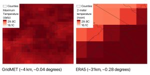
Regardless of which dataset is used, another consideration is how the resolution of the temperature data compares to the resolution of the health or socioeconomic data or outcome of interest. Using spatial resolution as an example, when a researcher wants to integrate temperature data to an administrative unit (say, county or municipality) associated with health records or survey respondents’ residence, they may care whether the temperature grid data in question is more or less coarse than those administrative units. At mismatched spatial scales, there may be implications for errors in measurement or attribution when averaging temperature into the administrative units. As an example, the figure below shows gridMET and ERA5 data for the same day (July 31, 2025) in the Philadelphia, PA and surrounding NJ area. Averaging across finer resolution data would likely be more suitable for finer-scale (smaller) units such as administrative units that represent urban areas and seen in the center of the figure below.
Finer scale data may also be more suitable when within administrative unit variation in temperature is high, or the analyst wants to capture that variation. For coarser administrative units, if additional information such as where population is concentrated is not available, use of the coarser temperature data may be as suitable as finer-grained data, noting of course that any sub-unit variation over these administrative areas is simply unobserved (Porter & Howell, 2016) or was reallocated with ancillary data (Zoraghein and Leyk, 2018, Uhl et al. 2018).
In the context of gridded population data, Leyk et al. (2019) provide a review of products available and a guide for understanding underlying data used in each gridded product, including the population data (spatial coarseness and how change over time is handled), use of ancillary data (such as settlements, roads or land cover), and methods used to allocate population within a defined grid “cell size”. All of these impact the suitability of use in particular applications. Fitness-for-use guidelines for these global population gridded dataset may depend on spatial and temporal resolution, scale and setting (rural vs urban), and mechanism of interest as noted in Leyk et al. (2019) and the same principles can act as a lens when evaluating which climate data set is most suitable for a given analysis.
Materials from a CACHE demonstration project “Heat, Disability in older adults and Care” from El Colegio de Mexico provides code and guidance for calculating UTCI using ERA5 data, producing municipality-level estimates of number of severe heat days: https://agingclimatehealth.org/severe-heat-days-using-the-universal-thermal-comfort-index/
References
Cruz, M., Mach, K. J., Turek-Hankins, L. L., Ashad-Bishop, K. C., Bailey, Z. D., Evans, S. D., Fanning, A., Fernandez-Burgos, M., Gilbert, J., Howard, B., Mahabir, M., Marturano, J., Murphy, L. N., Muse, N., Pérodin, J., & Clement, A. C. (2025). Where heat does not come in waves: A framework for understanding and managing chronic heat. Environmental Research: Climate, 4(2), 023002. https://doi.org/10.1088/2752-5295/adc827
Engel, R. E. Mackres, M. Palmieri and E. Anzilotti (2025). Beyond the Thermometer: 5 Heat Metrics That Drive Better Decision-Making, World Resources Institute Insights March 17, 2025 https://www.wri.org/insights/beyond-thermometer-measuring-heat
Leyk, S., Gaughan, A. E., Adamo, S. B., De Sherbinin, A., Balk, D., Freire, S., Rose, A., Stevens, F. R., Blankespoor, B., Frye, C., Comenetz, J., Sorichetta, A., MacManus, K., Pistolesi, L., Levy, M., Tatem, A. J., & Pesaresi, M. (2019). The spatial allocation of population: A review of large-scale gridded population data products and their fitness for use. Earth System Science Data, 11(3), 1385–1409. https://doi.org/10.5194/essd-11-1385-2019
Porter, J. R., & Howell, F. M. (2016). A spatial decomposition of county population growth in the United States: Population redistribution in the rural-to-urban continuum, 1980–2010. In Recapturing space: New middle-range theory in spatial demography (pp. 175-198). Cham: Springer International Publishing.
Uhl, J. H., Zoraghein, H., Leyk, S., Balk, D., Corbane, C., Syrris, V., & Florczyk, A. J. (2020). Exposing the urban continuum: implications and cross-comparison from an interdisciplinary perspective. International Journal of Digital Earth, 13(1), 22–44. https://doi.org/10.1080/17538947.2018.1550120
Zoraghein, H., & Leyk, S. (2018). Enhancing areal interpolation frameworks through dasymetric refinement to create consistent population estimates across censuses. International Journal of Geographical Information Science, 32(10), 1948–1976. https://doi.org/10.1080/13658816.2018.1472267