If you’re interested in contributing a short What Am I Reading post, we’d love to hear from you! Email us at cache@colorado.edu.
Written by Sophia Arabadjis, MA, MSc, PhD. Institute for Implementation Science in Population Health, City University of New York Graduate School of Public Health and Health Policy
Have you ever considered linking population data to information from a thematic map on, for example, coastal flooding, social mobility, wildfire hazard or social vulnerability? Maps are powerful communication tools, especially when interactive, allowing users to explore and visualize finely resolved geographies like ZIP code tabulation areas or census tracts or block groups. However, these maps and measures — and the data underlying them — are not always precisely measured, which can misconstrue spatial patterning of local risk and vulnerability.
These issues of measurement have very real implications for researchers and decision-makers who often use maps like these to provide environmental context or guide policy and resource allocation, respectively. Ignoring measurement issues can yield inaccurate insights.
This “What am I Reading?” entry provides an example of the implications of measurement error. Using material from our recent Annals of the American Association of Geographers paper, we explore how the sampling uncertainty in different data sources impacts wildfire vulnerability index construction. We describe various methods to construct vulnerability indices; discuss the sources of data used to create measures; and show how ignoring the sampling uncertainty can lead to false conclusions about vulnerability and a misallocation of resources[1].
Creating Composite Measures
In both academic literature and policy applications, it is common to summarize an area’s vulnerability using a singular score or number based on a scale or rubric, called a composite index. Composite indices are functions of several different measures recorded at each location or geographic unit across a landscape. Measures generally reflect population (social vulnerability components) and environmental context (locational vulnerability components) depending on the application. For example, the Center for Disease Control’s Social Vulnerability Index (SVI) combines national survey measures of socioeconomic status, household composition, racial and ethnic minority status, and local housing types/transportation to estimate overall vulnerability across a landscape[2]. For each location, or areal unit, the measures are summed to create a singular SVI score; scores between 0.75 and 1 indicate high vulnerability. The SVI and other similar composite indices (e.g. SoVI, SEDAC [3-6]) are increasingly used to prepare and direct resources towards areas in the top ~10% of scores, a.k.a. “highly vulnerable” areas[7-11].
Considering Measurement Error
While environmental measures may come from a variety of sources, the population measures are often from the same source: the American Community Survey (ACS). The ACS is a monthly survey of roughly 3.5 million people in the United States. The survey asks detailed questions about economic, social, and demographic characteristics, which are then aggregated (across areas and years) to different census geographies, from census block groups (600 – 3,000 people) all the way up to national estimates. Though 3.5 million people may seem like a large survey, this equates to roughly 14 people per census block group annually[12]. These small sample sizes mean that the errors within a given measurement may be quite large[12], which in turn means that the true value of the measurement could feasibly be any value within a large range of values — simply because of the sampling design.
Fortunately, along with the population measure point estimates (for example, the population of older adults in a given area), the ACS also provides an estimate of the uncertainty due to the sample design[12-13]. The ratio of the sampling uncertainty value to the point estimate, called the coefficient of variation, can give us a quick insight into the estimate’s precision. For example, suppose the ACS suggests that 15% of the population in a given census tract is above the age of 65 with a standard deviation of 1.8%; the ratio would be 0.018/0.15 = 0.12, which is a relatively low value, so we have relatively high confidence that ~15% of the population in that area is actually an older adult. However, if we have the same estimate with a standard deviation closer to 8%, then the ratio is over 0.5 and suddenly we have a lot less confidence that 15% of the population is accurate. Figure 1 maps the ACS coefficient of variation for a subset of urban census tracts and block groups in Santa Barbara County. A coefficient of variation (CV) greater than 0.12 is relatively good value; a CV of 0.5 or greater suggests much less confidence and more uncertainty. The table at right gives the percent of Census block groups that fall in each category for this urban subset. The maps show higher coefficient of variation values at smaller census block group geographies, which indicates more error within smaller geographic units.
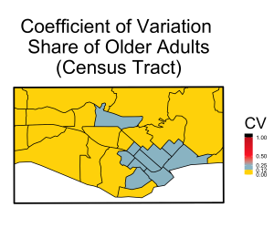
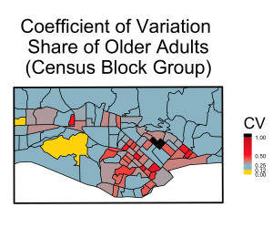
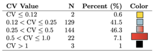
[Caption: Figure 1 maps the coefficient of variation (standard deviation/estimate) for a subset of urban Census tracts and Census block groups.]
Environmental measures also have uncertainties and measurement issues, though these generally take a different form. The error or noise in physical measurements may come mechanistic constraints of instruments (for example specificity and tolerance in thermometers), from spatial interpolation (e.g. creating a rain surface from point measurements across a landscape), or model-based variation (e.g. gridded outputs of complex physical or statistical models.) Some of these uncertainties may be knowable, such as the tolerance of an instrument, but others are not so easy to quantify.
Simulation is one way to propagate measurement error and assess its effects on the stability of findings. In a simulation framework, samples of each variable are repeatedly drawn from a range of acceptable values with an assumed shape (e.g. a normal distribution), and then summarized across those values. For example, one could take the pixel values of an environmental variable and the tolerance of that instrument and treat those as the mean and variance of normal distributions across a landscape (see Figure 2). Then, over the course of several samples (perhaps 1000), trends in values can be summarized. In our case, we are interested in how many times a specific pixel appears in the top 10% of values across each simulation. This is the recurrence rate and provides us insight into the stability of the top 10% of the distribution (“highly vulnerable”) areas.
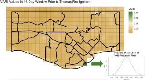
[Caption: Figure 2 Visible Atmospherically Resistant Index (VARI) is a satellite-derived measure that is closely correlated with live fuel moisture. Displayed are the VARI values per pixel in an urban area of Santa Barbara County in the period just before the Thomas Fire of 2017.[18]]
An example of the implications of sampling error using a wildfire risk index
To ground our investigation of wildfire risk, we chose the 2017 Thomas Fire as a case study. The Thomas Fire began December 4th, 2017 in Ventura County California and quickly spread into neighboring Santa Barbara County. Wildfires in this region of California are characterized by chaparral vegetation (burn-adapted shrublands), steep canyons, mesas, and unique wind patterns that make wildfires in this area both fast-moving and highly destructive[14-16]. By December 6th, 2024, the Thomas Fire had engulfed more than 100,000 acres; it would go on to consume 281,000 acres, destroy 1000 structures, and force more than 100,000 people to evacuate (see Figure 3)[17].
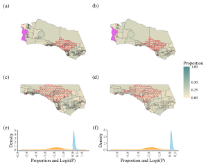
[Caption: Figure 3 The Thomas Fire final fire perimeter (red, hexagonal pattern) burned into densely populated coastal regions of Santa Barbara and Ventura counties (a-d). The estimated population aged 65 years or more per US Census block group (left column) and tract (right column) shows the proportion of older adults varies spatially across counties. Source: Arabadjis et al., 2025[1]]
With the Thomas Fire as our backdrop, we construct a simplified wildfire risk index with two measures common to the literature: a measure of the share of the population of older adults from the ACS (aged 65 years or older) and a satellite-based measure of vegetation moisture called the Visible Atmospherically Resistant Index (VARI). The VARI is derived from the green-to-red band signals and is strongly correlated with live fuel moisture which in turn, is strongly associated with wildfire ignition, spread and intensity in chaparral environments[18]. We take several steps.
First, we use a simulation framework within which samples are repeatedly drawn from the range of values (proportion of older adults) dictated by the sampling uncertainty. In mathematical terms, we take a draw from a normal distribution with mean as the logit-transformed point estimate ) and variance (specified from the variance estimate replicate tables for each Census geography (s). (See equation 1.)

We then summarize across the simulations to make sense of impacts of the sampling uncertainty of the ACS. We show that the selection of the top 10% most vulnerable areas — the areas that would likely be identified to receive resources — is sensitive to sampling uncertainty. We find that at smaller analytic scales (i.e. census block groups), the top 10% most vulnerable areas selected are not necessarily the same as if we took the proportion or share of older adults at face value.
Figure 4 provides a visual explanation of this finding, comparing the top 10% most vulnerable Census block groups (left column) and Census tracts (right column). Panels (a) and (b) show the top 10% areas according to the raw point estimates of the share of older adults in each area. Panels (c) and (d) show the recurrence rates of each Census block group or tract over the course of 1000 simulations. Areas shaded in brown-to-gold consistently appear in the top 10% most vulnerable (in 90+% of simulations); areas shaded in green-to-tan appear with less frequency in the top 10%, but any draw from the distribution is equally likely under the distributional assumptions. Panels (e) and (f) show the difference in the top 10% using the raw point estimates versus the simulation. Areas shaded in blue were ranked in the top 10% using the raw point estimates and the simulation. Areas in yellow were only ranked in the top 10% using the raw estimates, and areas in pink were only selected using the simulation method. Given the different sizes of Census tracts and block groups in Ventura and Santa Barbara county, these are difficult to see. For Census block group map (e), 2 areas are shaded pink; in the Census tract map (f) 1 area is shaded pink. These differences suggest that resources may be misallocated (or more resources may be needed). Areas in red are excluded from analysis.
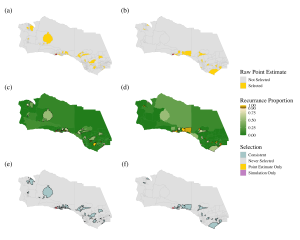
[Caption: Figure 4 displays the Census tracts (right) and Census block groups (left) of Santa Barbara and Ventura counties. In the top panel, geographies with a top 10% share of the older population are highlighted in yellow. In the middle panel (c-d) show the recurrence rates for the top 10% from the simulations. The lowest panel (e-f) maps differences in which geographies are in the top 10% of older adult population share by simulation versus raw point estimate. Source: Arabadjis et al., 2025[1]]
Second, we propose a statistical model and simulation procedure that combines the older adult population measure and the vegetation measure to create an example composite wildfire risk index. (See equation 2.) Importantly, our statistical model and procedure accounts for the sampling uncertainty of both the population and environmental measures and has a closed form expression of the variance[1]. (See paper for details.)

Similarly to Figure 4, each point in panels (c) and (d) in Figure 5 are colored to represent the proportion of simulations for which the index value at that point appeared in the top 10% of each sample (i.e. vulnerable areas). Areas in green almost never appeared in the top 10%; areas in tan appeared in the top 10% in roughly ⅔ or more of samples; and areas in brown-to-gold appeared in the top 10% in ninety percent or more of the simulations. These brown-to-gold areas are consistently highly vulnerable per our index.
Ultimately, our simulations show that accounting for the sampling design makes a difference in which areas are designated as “highly vulnerable to wildfire,” and that the uncertainty in the older adult measure likely dwarfs any uncertainty in the vegetation measure.
In this way, wildfire risk, in particular, would benefit from more finely resolved person-level data, such as parcel-level indicators from county tax assessor data and specialized survey data measuring risk, mitigation, and specific demographic indicators. This is especially important for older adults who may live in wildfire prone areas, but have different risk profiles in terms of knowledge, capacity, and underlying health[19].
Our results extend beyond our simplified wildfire example. We show that ignoring the sampling uncertainty in any ACS population estimates used in an index may misidentify risk across a landscape. We also note that the more complex the index (more measures), the more complicated the statistical model needs to be to incorporate the uncertainty, and the more trouble the subsequent risk distribution may be (multimodal, for instance).
However, simulation is another powerful tool that can help practitioners overcome sampling design constraints. Generating maps of simulation summaries (such as Figures 4 and 5) are potentially just as interpretable, but more true to the underlying unknowns in the data.
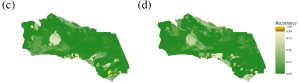
[Caption: Figure 5 maps the recurrence rates for each point (s) in the top 10% of wildfire risk index values. Subfigure (c) shows a Census block group-based-index and subfigure (d) shows a Census tract-based index. Source: Arabadjis et al., 2025[1]]
The article contributes to a robust and growing literature on vulnerability to environmental hazards. We show that uncertainty in the underlying data can distort vulnerability indices, especially as areal units get smaller. However, simulation is a pragmatic tool to help practitioners rigorously identify vulnerable areas and improve resources targeting across a landscape.
The real take-home message is that the next time you click on a map that highlights certain geographies as ‘highly vulnerable’, interpret with care!
References:
[1] Arabadjis, S. D., Zheng, Z., Strange, L. P., Murray, A. T., & Sweeney, S. H. (2026). Social Vulnerability, Locational Vulnerability, and Uncertainty in Wildfire Risk Index Construction. Annals of the American Association of Geographers, 116(5), 1211–1234. https://doi.org/10.1080/24694452.2025.2604851
[2] Flanagan, Barry E. et al. (2011). A Social Vulnerability Index for Disaster Management. 8(1).
[3] Cutter, S.L., B.J. Boruff, and W.L. Shirley. (2003). Social Vulnerability to Environmental Hazards. Social Science Quarterly 84(2). DOI: https://doi.org/10.1111/1540-6237.8402002
[4] Cutter, S.L. (1996) Vulnerability to Environmental Hazards. Progress in Human Geography 20(4). https://doi.org/10.1177/030913259602000407
[5] Cutter, S.L. (2024) The Origin and Diffusion of the Social Vulnerability Index (SoVI). International Journal of Disaster Risk Reduction. 109(104567). https://doi.org/10.1016/j.ijdrr.2024.104576
[6] NASA SEDAC. 2023. Center for International Earth Science Information Network (CIESIN) Documentation for the U.S. Social Vulnerability Index Grids: NASA Socioeconomic Data and Applications Center (SEDAC). New York. Columbia University.
[7] South Carolina Office of Resilience. (2026). Retrieved June 11, 2026, from https://scor.sc.gov/
[8] State of California Governor’s Office of Land Use and Climate Innovation (2026). Retrieved June 11, 2026, from https://vcp.lci.ca.gov/
[9] Federal Emergency Management Agency, FEMA (2026). Retrieved June 11, 2026, from https://www.fema.gov/emergency-managers/practitioners/recovery-resource-library/social-vulnerability-environmental
[10] U.S. Department of Agriculture and Rural Development, USDA (pre-2024). Retrieved 2024 from https://www.rd.usda.gov/priority-points/equity-search (No longer available.)
[11] Maine Infrastructure and Adaptation Fund MIAF (2026). Retrieved June 11, 2026 from https://www.maine.gov/future/climate/community-resilience-partnership and https://www.maine.gov/future/sites/maine.gov.future/files/inline-files/CAG2026-7-ProgramStatement.pdf
[12] Spielman, S. E., Folch, D., & Nagle, N. (2014). Patterns and causes of uncertainty in the American Community Survey. Applied Geography, 46, 147–157. https://doi.org/10.1016/j.apgeog.2013.11.002
[13] U.S. Census Bureau. (2017). Documentation for the 2013-2017 variance replicate estimates tables. https://www2.census.gov/programs-surveys/acs/replicate_estimates/2017/documentation/5-year/2013-2017_Variance_Replicate_Tables_Documentation.pdf
[14] Murray, A. T., Carvalho, L., Church, R. L., Jones, C., Roberts, D., Xu, J., Zigner, K., & Nash, D. (2021). Coastal Vulnerability under Extreme Weather. Appl. Spat. Anal. Policy, 14(3), 497–523. https://doi.org/10.1007/s12061-020-09357-0
[15] Park, I., Fauss, K., & Moritz, M. A. (2022). Forecasting Live Fuel Moisture of Adenostema fasciculatum and Its Relationship to Regional Wildfire Dynamics across Southern California Shrublands. Fire, 5(4), Article 4. https://doi.org/10.3390/fire5040110
[16] Storey, E. A., Stow, D. A., Roberts, D. A., O’Leary, J. F., & Davis, F. W. (2021). Evaluating Drought Impact on Postfire Recovery of Chaparral Across Southern California. Ecosystems, 24(4), 806–824. https://doi.org/10.1007/s10021-020-00551-2
[17] CAL FIRE. 2025. Statistics–CAL FIRE. https://www.fire.ca.gov/our-impact/statistics
[18] Peterson, S., D. Roberts, and P. Dennison. 2008. Mapping live fuel moisture with MODIS data: A multiple regression approach. Remote Sensing of Environment112 (12):4272–84. doi: 10.1016/j.rse.2008.07.012.
[19] De Fries, C., C. Melton, R. Smith, L. Reyes Mason. (2022). The Impacts of Wildfires on Older Adults: A Scoping Review. Innovation in Aging, 6:Supplement 1. https://doi.org/10.1093/geroni/igac059.2307
[20] National Interagency Fire Center. 2025. National Interagency Fire Center. https://data-nifc.opendata.arcgis.com